Cellular Automata
Cellular automata is a method of computation by which cells on a grid change state over time. Although the
grid types can vary, a common grid type is a two dimensional rectangular grid with the left and right edges,
and the top and bottom edges, considered adjacent (i.e. on an NxN grid, cell N+1 is the same as cell 0),
producing a torus. Each cell has a state where it contains one out of two or more values. For each cell in the
grid, rules are applied to determine
its state in the next time step. A rule usually determines the state of a cell in the next time step based on
the states of neighboring cells in the current time step. On a rectangular two dimensional grid,
common neighborhoods include the Von Neumann neighborhood (the 4 neighbors immediately adjacent to a cell
which differ in one coordinate from the cell - the North, South, East and West cells adjacent to the cell), and
the Moore neighborhood (the 8 neighbors which differ in one or two coordinates). As rules are applied and
time steps are performed, behaviour (computation) occurs on the grid.
Game of Life
The most well known cellular automaton is Conway's Game of Life. In a 1970 Scientific American article, John
Conway defined the system as follows:
The grid is 2 dimensional.
The Moore neighborhood is used for rule computation.
Each cell can be in only one of two states - "alive" or "dead" (occupied or empty).
The rules are as follows:
- A dead cell with three live neighbors becomes alive (is born) in the next time step.
- A live cell with two or three live neighbors stays alive in the next time step.
- In all other cases, a live cell dies in the next time step - it dies of lonliness if it has too few
neighbors, or of overcrowding if it has too many.
These rules, although simple, produce a wide variety of patterns (collections of cells), such as blinkers
(patterns which change to one state in the next time step, then back to their original state in the time
step after that), gliders (patterns which retain their shape but move across the grid), and eaters (patterns
which, when become in contact with other patterns, destroy them). These patterns seem to have a "life" of their
own.
Percolation
Cellular automata itself has many other applications beyond artificial life. In 1992, my senior research
project for my Physics degree was an application of cellular automata to spin systems. An idealized material
can be considered to have particles which have a magnetic spin in the "up" direction or in the "down" direction.
In an average material, the number of particles are distributed roughly evenly between up and down spins, so the
material itself has no net magnetic field. If either "up" or "down" spins predominate, a magnetic field is
present. It has been seen that the "becoming magnetic" as more of one type of spin is "added" to a material is
not a linear process - there is a "phase transition" at some point where the material suddenly becomes magnetic.
This phase transition can also be seen in other systems. Consider a network of interconnecting pipes and valves,
initially with all of the valves closed, and suppose there is a source of water at one end of the network. As
valves are turned on, water does not emerge from the other end of the network proportionally to the number of
open valves - only suddenly, when some percentage of the valves are open, is there a path from one end to the
other to let water flow. There is a sudden phase transition from "no water" to "water."
The question to ask is "at what percentage of open valves does the water start to flow?" i.e. "At what
percentage does the phase transition occur?"
The same idea can be applied to disease spreading in a forest (how dense do the trees need to be to allow the
disease to spread from one tree to another?), or turning an insulator into a conductor by adding particles of
conducting material (how much conducting material must be added for a conducting path to be present across the
insulator?).
This process can be simulated using a cellular automaton, as described in the
paper published
in the Proceedings of the Sixth Annual Conference on Undergraduate Research (NCUR) that was summarized from my
research project. Using much more current, and much faster, hardware, I recently performed a similar
simulation as before in order to illustrate the process.
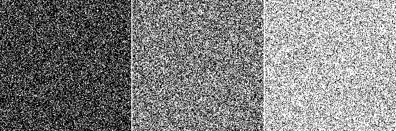
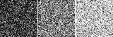
Step 1 - Randomization
The first step in the process is to randomly distribute particles on a grid at a specified concentration (i.e.
"A cell has a 10% chance of being present"). The images below show grids with initial distributions of 0.25,
0.50, and 0.75. The higher the concentration, the more densely packed are the "live" cells.
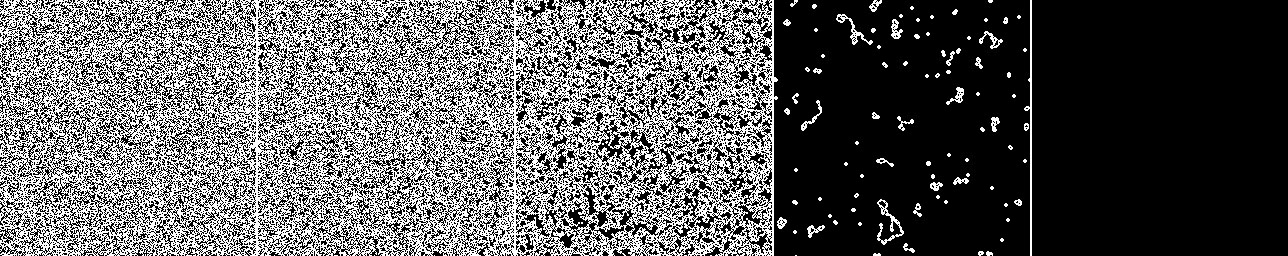
Step 2 - Settling
In order to simulate characteristics of different materials, a settling process is performed. A rule is applied
to the grid which states the following:
- If a cell is dead, it remains dead in the next time step.
- If a cell is alive and has more than N neighbors (Moore neighborhood), it becomes dead in the next time step,
otherwise it remains alive.
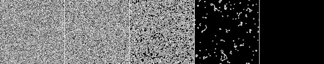
These rules are repeated until no more changes occur on the grid (it becomes "stable"). The images below
show the settling process for a grid with a randomization of 60% alive (.6), and N=1, N=2, N=3, N=4 and N=5.
Note that its not until N=3 that an easily observable change in the grid from its random state occurs. At N=4,
however, the grid has only disconnected blobs of cells, and for N=5, all cells have died (no patterns of
cells for which all cells in the pattern have 5 or more neighbors were produced in the randomization step).
One can also think of this step as simulating materials which clump together - the higher the N, the greater
the clumpiness. For instance, think of a small amount of water on a countertop. Rather than staying spread
out, surface tension tends to pull the water into small blobs - blobs not unlike the N=4 image above.
Step 3 - Spanning Cluster Detection
The determination of when the phase transition occurs can be viewed as when a cluster of living cells is large
enough so it spans the grid from one end to the other. The detection of this cluster can also be performed by
a cellular automaton rule, with a little preparation.
Initially, look at column 0 of the grid. If any cells are alive in that column, mark them blue. Once that
is done, apply the following rule until the grid is settled:
- If a live cell is adjacent (though consider the grid just as a grid - not as a torus) to a marked cell,
mark the live cell in the next time step.
- If a cell is live but not adjacent to a marked cell, or the cell is dead, it remains unmarked in the
next time step.
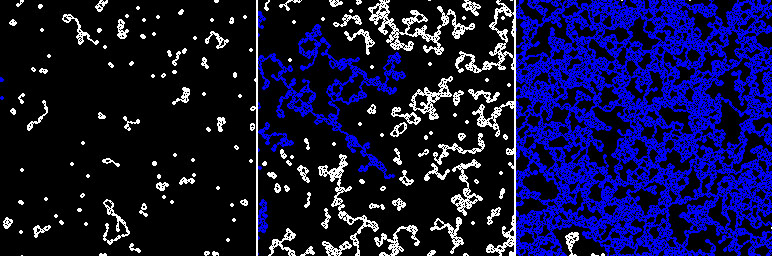
The images below are just before, and just after, a phase transition for N=4. The leftmost image is a
concentration of 60%. After the settling, almost no cells are present in column 0, and clearly no spanning
cluster is present. The center image is a concentration of 65%. A rather large cluster is present, though it
does not span the entire grid. The rightmost image is 70%. The cluster now spans the entire grid and the
phase transition has ocurred.

Summary of Results
For each concentration in 1% intervals (c), 20 random distributions were made, the settling process performed,
and a spanning cluster sought. p(c) is the percentage chance that for a given c a spanning cluster was found.
N from 1 to 5 are shown on the same graph, and although a different neighborhood was used, results similar to
the paper are present - as N increases, the phase transition point shifts to higher concentrations.